Recurrent Neural Networks (RNNs) explained

Sources

1. https://www.deeplearningbook.org/contents/rnn.html
2. https://arxiv.org/abs/1506.00019
3. https://arxiv.org/pdf/1312.6026.pdf
4. https://arxiv.org/pdf/1901.00434.pdf
5. https://www.researchgate.net/publication/228394623_A_brief_review_of_feed-forward_neural_networks

From Feedforward to RNNs

Recurrent Neural Networks (RNNs) are a class of neural networks designed to process sequential data, such as time series, text, audio, or any other type of sequential data. RNNs were developed to overcome the limitations of feedforward networks that don’t maintain a memory of past information.

Let’s take a general look at Feedforward Networks, to then better understand RNNs.

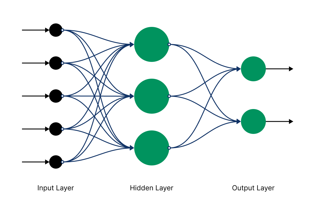
In feedforward networks, input is processed in a single pass, from input to output, without retaining any memory of previous inputs. Each input is treated independently from the others, making feedforward networks suboptimal for tasks requiring an understanding of data sequences or temporal contexts. This behavior is a direct consequence of the structure of a feedforward network: relatively simple and linear, with layers of neurons connecting directly one after the other in one direction, without cycles. Each layer receives input only from the previous layer and sends output only to the next layer. Feedforward networks are employed in specific areas, such as classification and regression tasks where the order of inputs isn’t relevant (image classification or predicting time-independent values).

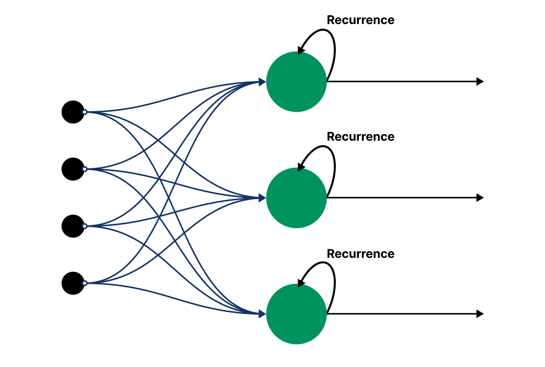
RNNs, unlike feedforward networks with unidirectional information flow and independent layer weights, feature recurrent connections enabling each hidden layer to be shaped by both the current input and the previous hidden state’s output. This creates an “internal memory”, useful for processing data sequences by allowing the network to consider past inputs, thus handling temporal dependencies. Ideal for tasks like language modeling, speech recognition, and sequence generation, RNNs use this memory to manage the sequence context, a key difference from the simpler feedforward approach. We will see their graphical visualization later, but first, a mathematical digression is useful to better understand how an RNN works.

RNNs Key Equations

In RNNs, there are multiple key equations and important mathematical concepts to understand. However, we will focus on the two most comprehensive equations for an RNN, which specify all the necessary calculations for computation at each time step on the forward pass in a simple recurrent neural network. $$h^{(t)}=\sigma(W^{hx}x^{(t)}+W^{hh}h^{t-1}+b_h)$$ This equation represents how the hidden state $h^{(t)}$ is updated at time $t$. Each hidden state is calculated based on three components:

1. The product of the weight matrix between the input and the hidden layer $W^{hx}$ and the input at time $t$, $x^{(t)}$.
2. The product of the recurrent weight matrix between the hidden layer and itself at adjacent time steps $W^{hh}$ and the hidden state at the previous time $t-1$, $h^{(t-1)}$.
3. The bias vector $b_h$.

The same equation can be interpreted in a slightly different and alternative way, as follows:

$$h^{(t)}=f(h^{(t-1)}, x^{(t)}; \theta)$$

These three terms are summed together and then passed through an activation function $\sigma$, such as the sigmoid function or the hyperbolic tangent, which updates the RNN’s hidden state $h^{(t)}$.

The purpose of the activation function is to introduce non-linearity into the model, allowing the model itself to represent complex and non-linear relationships between input and output variables.

The matrices mentioned in the formula are weight matrices that connect the previous hidden state to the current hidden state, the input to the hidden state, and the hidden state to the output. $$\hat{y}=softmax(W^{yh}h^{(t)}+b_y)$$ This equation is a typical representation of the output phase in an RNN, where the output $\hat{y}^{(t)}$ at time $t$ is calculated using the softmax function. In detail:

• $\hat{y}^{(t)}$ is the output predicted by the network at time $t$,
• $W^{yh}$ is the weight matrix that connects the hidden state $h^{(t)}$ to the output,
• $h^{(t)}$ is the hidden state at time $t$,
• $b_y$ is the bias vector associated with the output,
• the softmax function is an activation function used in multi-class classifications to transform scores (logits) into probabilities.

In an RNN, the softmax output $\hat{y}^{(t)}$ is often used to determine the probability of each possible next element in a sequence, such as the next word in a text. It can be used to evaluate performance during training or to generate new sequences during the inference process.

Design Patterns and Principles

Based on the definition we have given of RNNs, and in light of their computational structure, we can identify the following principles or design patterns of RNNs:

1. Cyclic Structure: Each unit of the RNN receives two inputs: the current element of the data sequence and the “hidden state” from the previous unit, which acts as a form of memory that carries information from one element to another in the sequence.
2. Hidden State: The hidden state is the heart of RNNs, allowing the network to accumulate knowledge throughout the sequence. Recurrent hidden layers leverage a cyclic memory mechanism that makes them “stateful,” allowing the network to accumulate knowledge over the sequence. At each time step, the hidden state is updated based on both the current input and the previous hidden state. This feature ensures that, alongside the evolution of the hidden layers, a hidden state is also developed, which is crucial for the RNN’s ability to process sequential information.
3. Shared Parameters: Unlike feedforward networks, where each layer has its own set of parameters, in an RNN, the same set of parameters (weights) is used at every time step. This concept is known as “shared parameters” and allows the RNN to process sequences of variable length with a fixed model.
4. Sequential Structure: RNNs are designed to work with sequential data, and their architecture reflects this characteristic. Inputs are processed one after the other, and the output from one step can influence the processing of the next.
5. Output: At each time step, the RNN can produce an output based on the current hidden state. The output can be generated at each step (for example, in language modeling) or only at the end of the sequence (for example, in sequence classification).

With an understanding of the fundamental building blocks of RNNs, we now delve into their computational representation.

Computational Graph and Backpropagation

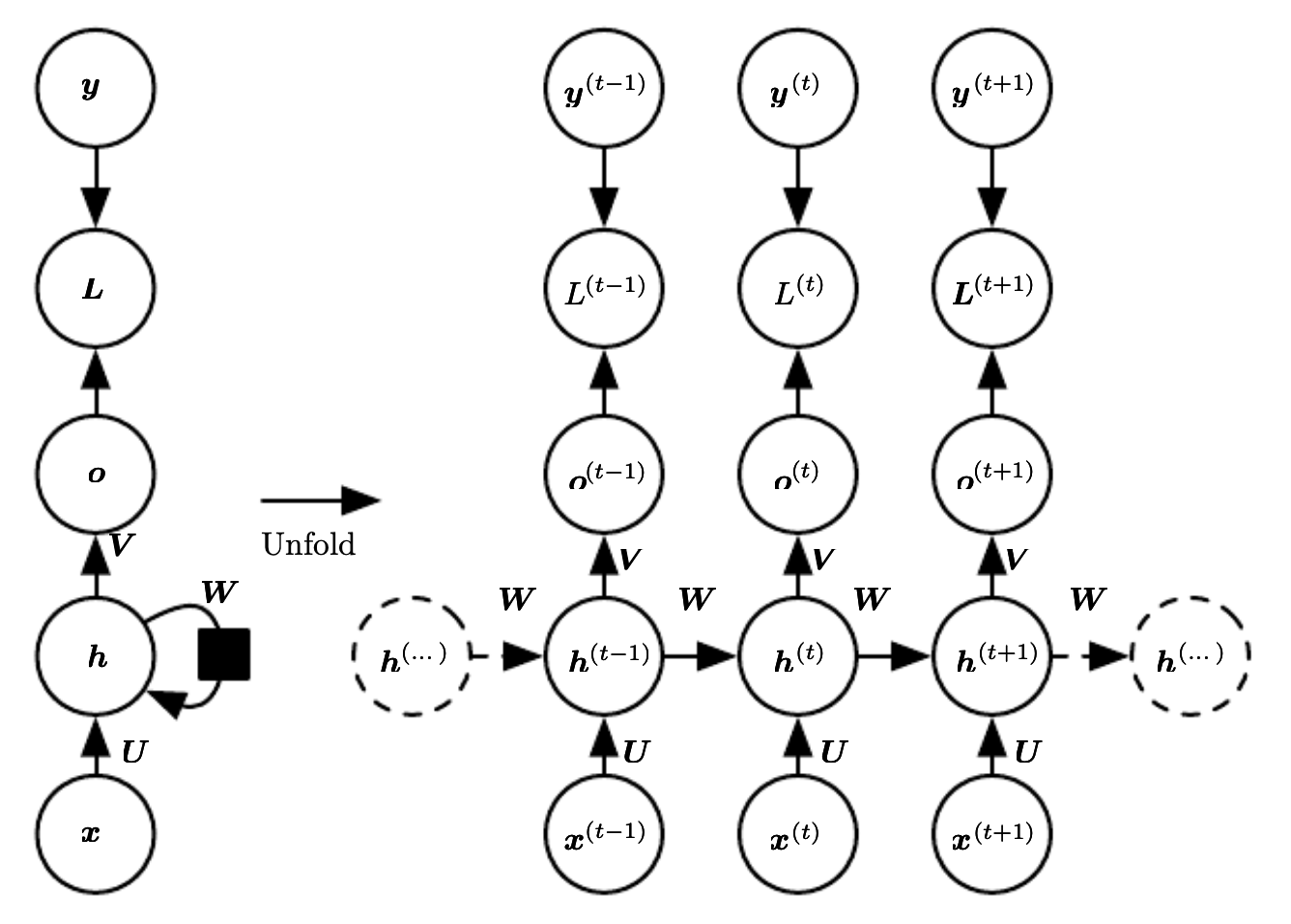
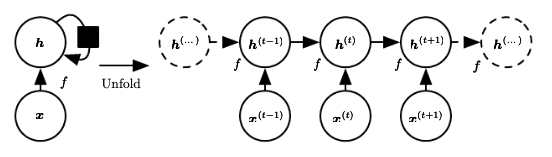
It is important to delve deeper into the concept of unfolding. In the context of RNNs, the term unfolding refers to the process of transforming the recurrent network, which intrinsically has a cyclic structure due to its hidden state passing from one time step to the next, into an extended (or unfolded) version that displays the entire sequence of operations across time steps. This unfolding transforms the cyclic structure into a chain of replicas of the network, one for each time step in the sequence, making evident how information flows through the time steps.

Following the concept of unfolding, it’s essential to examine Backpropagation Through Time (BPTT): it is an algorithm that emerges as a variant of the standard feedforward Backpropagation algorithm, specifically designed for the training of RNNs. This variation of the standard algorithm is the necessary consequence of the recurrent nature of RNNs, which requires a different approach for the calculation of gradients and for the updating of weights during the training process.

The BPTT algorithm works by following these steps:

1. Unfolding the network: as we have previously seen, the RNN is unfolded over time to transform it into a feedforward network. This allows treating the temporal dependency between sequential inputs as connections within a larger network.
2. Forward propagation: the input is fed through the unfolded network, and the output is calculated for each time step.
3. Error calculation: the error (the difference between the expected value and the actual one) for each output in the sequence is calculated.
4. Backward error propagation (Backpropagation): the error is propagated backward to calculate the gradients of the weights relative to the error. This is the most critical step for training, as it determines how to modify the weights to reduce the error.
5. Weight update: finally, the weights are updated based on the calculated gradients. Stochastic Gradient Descent is typically used as the optimization algorithm.

Stochastic Gradient Descent (SGD) is a variant of the Gradient Descent algorithm, which is a technique for minimizing the cost (or loss) function associated with a model, i.e., the measure of how “far” the model is from making accurate predictions. I believe I will write a dedicated blog post on the topic. For now, we mentioned it only to connect to the next paragraph, where we will address the problem of Vanishing/Exploding Gradient, the major limitation of RNNs.

Vanishing/Exploding Gradient Dilemma

The problem of vanishing gradients and exploding gradients are two significant challenges in training RNNs, especially when working with very long sequences. These issues affect an RNN’s ability to learn long-term dependencies between elements in a sequence. Let’s look in detail at what these problems entail and how they manifest.

The vanishing gradient problem occurs when the gradient (the derivative of the loss function with respect to the network’s weights) tends towards zero during the backpropagation process. In RNNs, this is particularly problematic for long-term dependencies because of the repeated multiplication of small gradients across timesteps during BPTT. This can result in a gradient that becomes extremely small. Consequently, the weight update becomes insignificant, effectively rendering the network unable to learn from inputs that are distant in time. For this reason, the network may struggle to learn and retain information from earlier parts of the sequence.

Conversely, the exploding gradient problem occurs when gradients become excessively large during backpropagation. This can lead to overly large weight updates, causing instability in the network and making the training process diverge. In RNNs, this is often due to the repeated multiplication of large gradients across timesteps, which can exponentially increase the gradient’s value as it is backpropagated in time.

To overcome this issue, various techniques have been adopted that led to the development of new neural networks, such as Long Short-Term Memory (LSTM) networks. LSTMs were designed as a specific type of RNN cell with additional gating mechanisms, allowing them to selectively remember or forget information based on its relevance. These gating mechanisms help preserve important long-term dependencies in the hidden state vector and enable LSTMs to better handle sequences with long-term dependencies than traditional RNNs.

Ending

I’ve tried to explain clearly and summarize the most important points about RNNs. I dedicated a blog post to RNNs because I consider them important and foundational for the study of subsequent models, like Transformers. Anyway, even though traditional RNNs face difficulties in capturing long-term dependencies, variants like LSTM and GRU have been developed to overcome these limits. To understand and use them, I believe it’s necessary to know how RNN architectures are constructed.

Thank you for reading!

If you notice any inconsistencies, please send me an email at simone.bellavia@live.it, so I can make the correction.

If you enjoyed this blog post, consider following me on X/Twitter, @sineblia.